TAQ Project in Python#
In this project, we’ll use the NYSE Trade and Quote (TAQ) database on WRDS described here: https://wrds-www.wharton.upenn.edu/pages/about/data-vendors/nyse-trade-and-quote-taq/. This is our workflow:
Select a company and a trading date. Fetch stock price data for this company by the second.
Obtain the five-minute average stock price for each observation (not a rolling average) as a new table.
Merge the two tables.
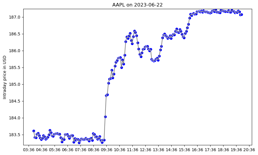
Graph the time series for the stock prices with the five-minute average indicated by blue dots.
To get started, we’ll first load our python libraries and then establish a WRDS connection.
# import packages
import wrds
import pandas as pd
import matplotlib.pyplot as plt
import matplotlib.dates as mdates
import seaborn as sns
# wrds connection
conn = wrds.Connection(wrds_username='best-user-ever')
Loading library list...
Done
1. Obtain WRDS data table#
Select a company and date to use in this example.
# inputs for a date and ticker
dd = '20230622'
stock = "AAPL"
Submit a sql query.
# Create the SQL query to get a table from the TAQ database
sql = f"""
SELECT CONCAT(date, ' ', time_m) AS DT,
       ex, sym_root, sym_suffix, price, size, tr_scond
FROM taqmsec.ctm_{dd}
WHERE (ex = 'N' OR ex = 'T' OR ex = 'Q' OR ex = 'A')
  AND sym_root = '{stock}'
  AND price != 0 AND tr_corr = '00'
"""

# Execute the query
df_aapl = conn.raw_sql(sql)

# print the column names
print(df_aapl.columns)

# print the number of columns and rows
print(df_aapl.shape)
Index(['dt', 'ex', 'sym_root', 'sym_suffix', 'price', 'size', 'tr_scond'], dtype='object')
(111590, 7)
2. Obtain 5-minute averages#
# Convert the 'dt' column to datetime
df_aapl['dt'] = pd.to_datetime(df_aapl['dt'])

# Round 'dt' to the nearest 5-minute mark
df_aapl['dt'] = df_aapl['dt'].dt.round('5Min')

# Set 'dt' as the index
df_aapl.set_index('dt', inplace=True)

# Resample to get the average price every five minutes
df_aapl_resampled = df_aapl['price'].resample('5Min').mean()


# print the number of observations
print(df_aapl_resampled.shape)
(193,)
3. Merge Tables#
# Reset the index of both DataFrames
df_aapl.reset_index(inplace=True)
df_aapl_resampled = df_aapl_resampled.reset_index()

# Rename the column in df_aapl_resampled to avoid a naming conflict during the merge
df_aapl_resampled.rename(columns={'price': 'avg_price'}, inplace=True)

# Merge the two DataFrames
df_aapl = df_aapl.merge(df_aapl_resampled, on='dt', how='left')

# Fill NaN values in the 'avg_price' column
df_aapl['avg_price'] = df_aapl['avg_price'].ffill()

# print the column names
print(df_aapl.columns)

# print the number of columns and rows
print(df_aapl.shape)
Index(['dt', 'ex', 'sym_root', 'sym_suffix', 'price', 'size', 'tr_scond',
       'avg_price'],
      dtype='object')
(111590, 8)
4. Graph Results#
# Create a new figure
plt.figure(figsize=(10, 6))

# Plot the price series
sns.lineplot(x='dt', y='price', data=df_aapl, color='gray')

# Plot the aggregated price series
sns.scatterplot(x='dt', y='avg_price', data=df_aapl, color='blue', s=50)

# Set the x-axis label
plt.xlabel('')

# Set the y-axis label
plt.ylabel('Intraday price in USD')

# Set the y-axis limits
plt.ylim(df_aapl['price'].min(), df_aapl['price'].max())

# Set the x-axis major ticks to 60-minute intervals
plt.gca().xaxis.set_major_locator(mdates.MinuteLocator(interval=60))

# Set the x-axis major tick labels to the format HH:MM
plt.gca().xaxis.set_major_formatter(mdates.DateFormatter('%H:%M'))

# Set the title of the plot
plt.title(f'AAPL on {df_aapl["dt"].dt.date.unique()[0]}')

# Show the plot
plt.show()